This document is my personal deep-dive into how modern open-source GPT-style language models are actually built. It’s not meant to be a full survey of the literature; instead, it captures the pieces that helped me build an intuition for these models: how text becomes vectors, how positional information is injected, how attention is optimized, and how FFN variants like MoE increase capacity without blowing up compute.
1. Tokenization & Embeddings
The journey from human-readable text to a format the model understands begins here.
1.1. Tokenization:
- First, raw text is converted into a sequence of integers called “tokens” using a tokenizer (e.g., Byte-Pair Encoding or BPE, as mentioned in
tokenization.md). - This process breaks down words into common sub-words. For example,
tokenizationmight become["token", "ization"]. This allows the model to handle unknown words and understand morphological similarities (e.g.,run,running). - The set of all possible tokens forms the model’s vocabulary.
- First, raw text is converted into a sequence of integers called “tokens” using a tokenizer (e.g., Byte-Pair Encoding or BPE, as mentioned in
1.2. Token Embeddings:
- Process: Each token ID is mapped to a high-dimensional vector.
Input Text: "Hello world" Token IDs: [15496, 995] Embeddings: [[0.1, -0.2, ...], [0.4, 0.9, ...]] // Each vector has dimension `d_model` (e.g., 2880) - Goal: To represent tokens in a continuous vector space where semantic relationships are captured by distance and direction.
- Learned, Not Pre-trained: These embedding vectors are initialized randomly and are learned parameters. During training, the model adjusts them via backpropagation to place semantically similar tokens closer together. This is far more powerful than using static, pre-trained embeddings like Word2Vec because the meanings become contextualized to the model’s task.
- Process: Each token ID is mapped to a high-dimensional vector.
2. Positional Information: Rotary Positional Embeddings (RoPE)
2.1 Why Transformers Need Positional Information
As we try to understand positional embeddings, it helps to first ask why they exist at all. The self-attention mechanism by itself is position-invariant: if you shuffle the tokens and apply the same shuffle to Q, K and V, you get the same outputs, just shuffled. The math has no built-in notion of “first token”, “second token”, or “this token is 3 steps after that one”.
That’s a problem, because in language the order of tokens carries meaning. We want the model to know not just what the tokens are, but also where they appear and how far apart they are. To fix this, the Attention Is All You Need paper introduced positional encodings: extra information that we add to the token embeddings so that attention can take order into account.
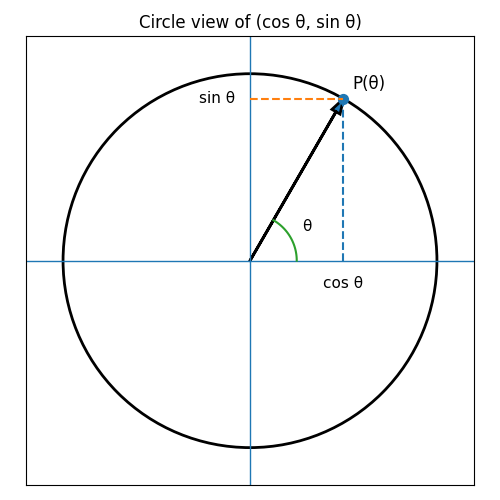
2.2 Sinusoidal Positional Encodings – Circle and Wavelength Intuition
The original Transformer uses sinusoidal positional encodings. The idea is to associate each position index pos with an angle $\theta$, and then use $(\cos \theta, \sin \theta)$ as a 2-D code. You can visualize this as a point moving around a unit circle:
- each position
poscorresponds to some angle $\theta(\text{pos})$ - the x-coordinate is $\cos \theta(\text{pos})$
- the y-coordinate is $\sin \theta(\text{pos})$
Different dimensions of the positional encoding use different “speeds” around this circle, controlled by a wavelength $\lambda$. A smaller $\lambda$ means that as pos increases, $\theta = \text{pos} / \lambda$ grows faster, so the point spins around the circle more quickly (higher frequency). A larger $\lambda$ means a slower rotation (lower frequency). Across all dimensions you get a mix of high- and low-frequency waves over position.
The key bit is what happens when you move from position pos to position $\text{pos} + k$. On the circle, that is just a rotation by a fixed angle that depends only on $k$. So the code at $\text{pos} + k$ is the code at pos rotated by a fixed amount. Because of this, linear layers can learn to detect relative offsets (“how far apart are these two positions?”) just by looking at how their sin/cos coordinates relate. That’s what people mean when they say sinusoidal encodings make it easier for the model to attend by relative position, even though we only ever feed in absolute indices.
2.3 Rotary Positional Embeddings (RoPE) – What GPT OSS Actually Uses
The Core Idea: Instead of adding positional information to the token embedding, RoPE encodes positional information by rotating the Query and Key vectors. The amount of rotation depends on the token’s absolute position in the sequence.
How It Works: Vector Rotation
Pairing Dimensions: The
d-dimensional Query and Key vectors are viewed as a sequence ofd/2two-dimensional vectors. For a vectorv, this would be[(v_0, v_1), (v_2, v_3), ..., (v_{d-2}, v_{d-1})].Defining Frequencies: A set of
d/2different angular frequencies (or “wavelengths”)theta_iare defined. These are fixed and not learned, typically set totheta_i = 10000^(-2i/d). This means the first pairs rotate slowly (long wavelength) and later pairs rotate quickly (short wavelength).Applying Rotation: For a token at position
m, each 2D pair(v_i, v_{i+1})is rotated by an angle ofm * theta_i. This is done using a 2D rotation matrix:This operation is applied to both the Query vectorqand the Key vectorkbefore the attention score is calculated.[x'_i] [cos(m*theta_i) -sin(m*theta_i)] [x_i] [x'_{i+1}] = [sin(m*theta_i) cos(m*theta_i)] [x_{i+1}]
The Magic: Encoding Relative Position The brilliance of RoPE is that the dot product between a rotated query
q'at positionmand a rotated keyk'at positionndepends only on their relative distancem-n.- Derivation Sketch: The dot product
q'_m · k'_ncan be expanded using the rotation matrix formula. After applying trigonometric identities (likecos(A-B) = cosAcosB + sinAsinB), the terms involving the absolute positionsmandncancel out, leaving a function that depends only on the original vectorsq,k, and the relative positionm-n. - Result: The attention score between
q_mandk_nbecomes a function of their content and their relative distance, which is exactly what we want.
- Derivation Sketch: The dot product
Key Advantages:
- Relative Position Encoding: It naturally captures relative positional information, which is more intuitive for language.
- Good Extrapolation: Because it’s not tied to a fixed-length learned embedding, RoPE can generalize better to sequence lengths longer than those seen during training.
- Stability: Rotation is a norm-preserving operation, meaning it doesn’t change the length of the vectors, which helps maintain training stability.
2.4 Comparing different positional encoding schemes
| Feature | Absolute (Traditional) | Relative | Rotary (RoPE) |
|---|---|---|---|
| Method | Add a vector to the token embedding | Add a bias to the attention scores | Rotate the token’s Q/K vectors |
| Analogy | House numbers (“House #5”) | Directions (“3 steps left”) | Clock angles (“angle difference”) |
| Generalization | Poor (struggles with unseen lengths) | Good (invariant to shifts) | Excellent (naturally encodes relative distance) |
| Complexity | Low (simple addition) | High (pairwise distance computation) | Medium (rotation via small matrix multiplies) |
3. RMS Normalization (RMSNorm)
A simple and efficient normalization layer used throughout the transformer blocks to stabilize training.
- Formula:
$$ \text{output} = \frac{x}{\text{RMS}(x)} \cdot g \quad \text{where} \quad \text{RMS}(x) = \sqrt{\frac{1}{d}\sum_{i=1}^{d} x_i^2 + \epsilon} $$
xis the input vector,g(gain) is a learned parameter vector, andepsilonis a small constant for numerical stability.- Advantages over LayerNorm:
- Simplicity & Speed: By omitting the mean-centering step of LayerNorm (
x - mean(x)), RMSNorm is computationally simpler and faster (~7-14% on GPUs). - Equivalent Performance: In practice, for large transformer models, the centering operation provides little to no benefit, and RMSNorm performs just as well or better. The network can implicitly learn to offset values if needed.
- Simplicity & Speed: By omitting the mean-centering step of LayerNorm (
4. The Transformer Block
The core repeating unit of the model. A model is a deep stack of these blocks. A single block consists of two main sub-layers: an attention mechanism and a feed-forward network.
4.1. Attention Sub-Layer
This layer allows tokens to “look at” and gather information from other tokens in the sequence.
- Optimized Attention Variants: To manage the computational and memory costs of standard Multi-Head Attention (MHA), modern models use more efficient variants.
| Variant | Query (Q) Heads | Key (K) Heads | Value (V) Heads | Benefit |
|---|---|---|---|---|
| Multi-Head (MHA) | N | N | N | High model quality, high memory cost. |
| Multi-Query (MQA) | N | 1 | 1 | Drastically reduces KV cache size, fastest inference. |
| Grouped-Query (GQA) | N | G (e.g., 4) | G (e.g., 4) | A balance between MHA’s quality and MQA’s speed. |
- Sliding Window Attention (SWA): To handle very long sequences efficiently, some models employ SWA. Instead of allowing every token to attend to every other previous token (which has a quadratic
O(n^2)cost), SWA restricts each token to only attend to a fixed-size window of recent tokens (e.g., the last 4096 tokens).
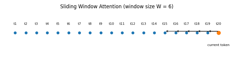
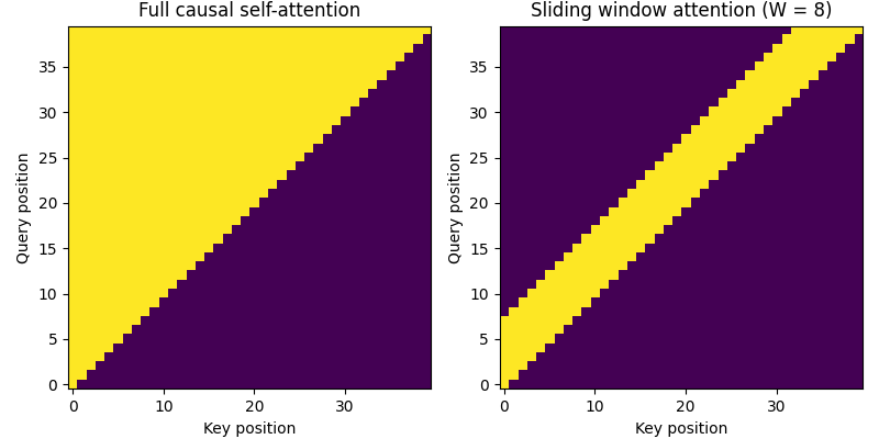
Benefit: This reduces the computational complexity to O(n * w), where w is the window size, enabling the model to process much longer contexts with a linear cost.
- Example: The Mistral 7B model is a prominent example that uses Sliding Window Attention to achieve a large effective context window while maintaining high efficiency.
- Interaction with KV Cache: SWA’s most significant impact is on the KV Cache. Instead of growing indefinitely, the cache becomes a fixed-size rolling buffer. It only needs to store the keys and values for the last
wtokens. When a new token is generated, the oldest token’s K/V pair is discarded, and the new one is added. This keeps memory usage constant and bounded, regardless of the total sequence length.
4.1.1 Information Propagation Beyond the Sliding Window
A common question about SWA is: if a token can only see the last W tokens, isn’t all prior information lost? The answer is no, due to a transitive information flow. Information from outside the window is not accessed directly, but its essence is carried forward through two mechanisms:
Horizontal Propagation (Token-to-Token):
- The token at position
Nattends to the token at positionN-1. - The token at
N-1has already attended to the token atN-2, and so on, back toN-W. - Therefore, the representation of token
N-1contains a summary of its own attention window. When tokenNattends toN-1, it indirectly accesses this summarized information. This creates a “ripple effect” where the semantic context is passed down from one token to the next.
- The token at position
Vertical Propagation (Layer-to-Layer):
- This effect is amplified across the model’s layers. The output representation of a token from Layer 1, which has gathered information from its local window, becomes the input to Layer 2.
- In Layer 2, when a token attends to its neighbors, it’s attending to representations that have already summarized information from the previous layer.
- Because of this, the “effective receptive field” of a token grows with each layer. By the final layer, a token’s representation has been influenced by information that originated far outside its immediate
W-sized attention window.
- KV Cache Size Impact: The choice of attention mechanism directly impacts the size of the KV Cache. MQA and GQA reduce the cache size by reducing the number of K/V heads. SWA reduces it by limiting the sequence length dimension of the cache.
4.1.2. Attention Bias
- Definition: The attention logits are computed as
attn_logits = (Q @ K^T) * scale + bias, wherebiasis added before the softmax and can be broadcast across heads and/or sequence positions.- Typical shapes:
[num_heads, 1, seq_len, seq_len],[1, seq_len, seq_len], or block-sparse masks.
- Typical shapes:
- Common uses:
- Causal Masking: Setting scores for future tokens to
-infinityto prevent a token from “cheating” and seeing the future. This is essential for auto-regressive generation. - Attention Linear Bias (ALiBi) (linear distance penalty): Implementing alternative positional encoding schemes like ALiBi (Attention with Linear Biases), where the bias penalizes attention between distant tokens.
- Relative position bias (T5-style): Learned bucketed biases that favor nearby tokens without explicit rotations.
- Segment/turn/document biases: Down-weight cross-segment attention (e.g., between chat turns) or up-weight separators.
- Task-specific nudges: Small positive bias to encourage attending to prefixes, BOS, or special control tokens.
- Causal Masking: Setting scores for future tokens to
- Implementation notes:
- The bias is added additively and can be static (no gradients; e.g., causal mask, ALiBi) or learned.
- Works independently of RoPE/MQA/GQA and with FlashAttention by fusing masks/biases into the softmax kernel.
- Memory cost is minimal due to broadcasting; compute overhead is negligible.
4.1.3. Attention Sinks
- Intuition: Reserve a small number of early positions (e.g., the first
mtokens) as “sink” tokens that every query can always attend to. These serve as stable anchors that preserve global context, especially under streaming or sliding-window inference. - Why it helps:
- Prevents quality drop when tokens outside the current window are no longer directly visible.
- Provides a consistent fallback target, stabilizing attention distributions and downstream normalization statistics.
- Acts like a “heat sink”: it can absorb a small, consistent fraction of attention mass to avoid brittle sparsity.
- Mechanism:
- Keep the K/V for the sink positions permanently in the KV cache, even when using SWA that evicts old tokens.
- Add a small positive bias
+b_sinkto logits targeting sink indices so that they receive a modest probability mass after softmax (e.g., 1–5%). - Optionally insert dedicated sink tokens (or reuse BOS) with embeddings tuned for summarization/aggregation.
- Practical guidance:
- Choose
min the range 1–4; setb_sinkto achieve a small but nontrivial attention share. - Can be introduced at inference-time only, but works best if the model is trained or finetuned with sink behavior.
- Compatible with RoPE, MQA/GQA, SWA, and FlashAttention.
- Choose
- Reference: Efficient Streaming of Language Models with Attention Sinks (arXiv:2309.17453).
# Pseudocode (inference-time biasing with m sink tokens)
def add_attention_bias(attn_logits, sink_indices, b_sink):
    # attn_logits: [batch, heads, q_len, k_len]
    # sink_indices: list/tensor of length m with K-side positions to favor
    attn_logits[..., sink_indices] += b_sink
    return attn_logits

# With sliding-window caching: always retain K/V at sink_indices
def update_kv_cache(cache, new_k, new_v, sink_indices, window_size):
    # Keep sinks + last (window_size - len(sink_indices)) positions
    retained = concat(cache.kv_at(sink_indices), cache.kv_last(window_size - len(sink_indices)))
    cache.k, cache.v = roll_and_append(retained, new_k, new_v)
    return cache
4.2. Feed-Forward Network (FFN) Sub-Layer
This is where the model does much of its “thinking” and knowledge recall.
Standard FFN: A simple two-layer MLP:
FFN(x) = ReLU(x @ W1 + b1) @ W2 + b2.SwiGLU Variant: Modern models often use a more advanced variant called SwiGLU (Gated Linear Unit with a Swish/SiLU activation) for better performance.
SwiGLU(x) = (SiLU(x @ W1) * (x @ W_gate)) @ W2- It uses three weight matrices instead of two. The gating mechanism (
x @ W_gate) allows the network to dynamically control how much information flows through the main path, leading to improved training and final model quality.
- It uses three weight matrices instead of two. The gating mechanism (
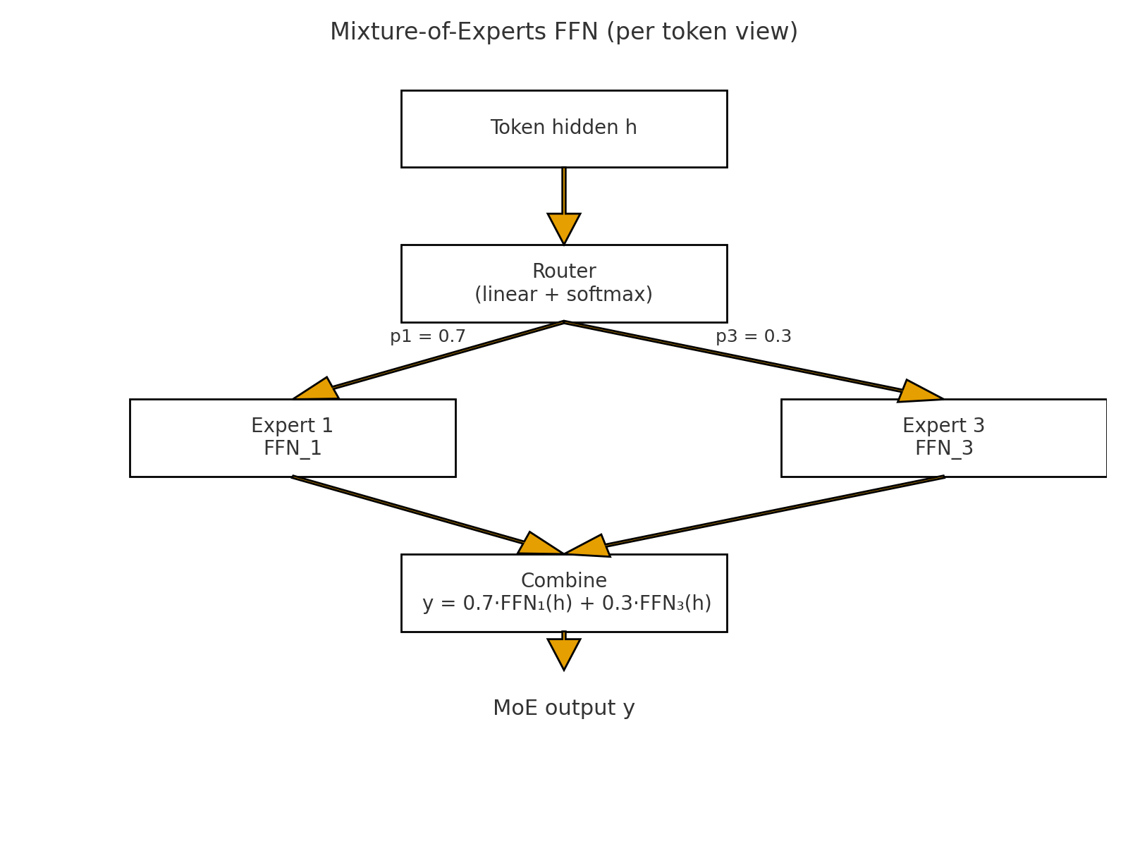
Mixture of Experts (MoE): To scale up model size efficiently, the FFN sub-layer can be replaced with an MoE layer.
- Architecture: Instead of one large FFN, there are multiple smaller FFNs (the “experts”).
- Routing: A small “gating network” or “router” (a simple linear layer + softmax) looks at each token’s hidden state and outputs probabilities for which expert should process it.
- Sparse Activation: Typically, only the top-2 experts are chosen for each token. The final output is a weighted sum of the outputs from these two experts.
- Benefit: This allows for a massive increase in the total number of parameters in the model, while the computational cost per token remains constant. A “load balancing loss” is often added during training to ensure all experts are utilized.
Load Balancing Loss – My Mental Picture
Mixture-of-Experts only helps if different experts actually get used. In practice, the router tends to fall in love with a few “easy win” experts early in training and send almost every token to them. Those experts get lots of gradient updates and become even better, while the others starve and never learn anything useful. This is called router collapse.
To prevent that, modern MoE layers add a small auxiliary load balancing loss. Over a batch of tokens, we look at two things for each expert:
- how much the router wants to use that expert (its average routing probability), and
- how many tokens actually go to that expert (its share of the routed tokens).
The load balancing loss pushes these quantities toward being roughly uniform across experts. Intuitively, it penalizes solutions where one expert is overloaded and others are idle. The main language modeling loss still decides what each expert should learn, but the load balancing loss makes sure every expert gets a steady stream of training data instead of the router sending everything to a single “favorite” expert.
4.3. Residual Connections
Residual connections (or “skip connections”) are the architectural glue that holds the transformer block together and, more importantly, allows the model to be trained at great depths.
How it Works: A residual connection is a direct data path that bypasses a sub-layer (like attention or FFN). The output of the sub-layer is then added to the original input that went into it.
output = input + SubLayer(LayerNorm(input))Why They Are Critical:
- Combating Vanishing Gradients: This is the primary reason for their existence. In very deep networks, gradients can shrink exponentially as they are propagated backward from the final layer to the initial layers. This causes the early layers to learn extremely slowly or not at all. The residual connection acts as an “information superhighway,” allowing the gradient to flow directly and unimpeded back through the network. This ensures that even the earliest layers receive a strong learning signal.
- Preserving Information: Each sub-layer transforms its input. The residual connection guarantees that the original, untransformed information from the beginning of the block is carried forward. The sub-layer’s job is simplified: it only needs to learn the residual—the change or update that should be applied to the original vector—rather than the entire transformation from scratch. This makes learning easier and prevents information loss.
Without residual connections, training transformers with dozens or hundreds of layers would be practically impossible.
5. Key-Value (KV) Cache
A critical optimization that makes auto-regressive text generation practical and fast.
- The Problem: During generation, to predict token
N+1, the model needs to attend to all previous tokens1...N. Naively re-calculating the Key (K) and Value (V) vectors for the entire context at every single step is computationally prohibitive. - The Solution: The KV cache is a memory buffer that stores the K and V vectors once they are computed.
- Step 1: Process prompt “The cat”. Compute and cache
K_the,V_the,K_cat,V_cat. - Step 2: Generate next token. Let’s say it’s “sat”. The model computes
Q_satand attends to the cached[K_the, K_cat]and[V_the, V_cat]. - Step 3: After generating “sat”, compute
K_satandV_satand append them to the cache. The cache now holds K/V for “The cat sat”. - Note: With Sliding Window Attention, this cache would be a fixed-size rolling buffer rather than an ever-growing list (see section 4.1).
- This turns a quadratic operation (recomputing everything) into a linear one (computing for one new token), making generation feasible for long sequences.
- Step 1: Process prompt “The cat”. Compute and cache
6. Overall Architecture & Workflow
Putting it all together, a GPT-style model processes data roughly like this:
Input
Raw text is passed to the tokenizer, producing a sequence of token IDs.Embedding layer
Token IDs are converted into token embeddings. Positional information (e.g., RoPE) is applied to the Q/K projections inside attention layers.Transformer blocks (stacked L times)
The sequence is processed throughLidentical blocks. For each block:a. Pre-attention norm
x_norm1 = RMSNorm(x)b. Attention
attn_out = GQA(Q = x_norm1, K = x_norm1, V = x_norm1)
(with RoPE applied to Q and K, plus any attention bias, SWA masking, sinks, etc.)c. First residual
x_res1 = x + attn_outd. Pre-FFN norm
x_norm2 = RMSNorm(x_res1)e. Feed-forward / MoE
ffn_out = MoE(x_norm2)(or a SwiGLU FFN in non-MoE models)f. Second residual
x = x_res1 + ffn_out
(thisxbecomes the input to the next block)Final projection
a. Apply a final RMSNorm to the last block’s output.
b. Use a linear layer (the LM head) to project to vocabulary size, producing logits for each token position.Softmax & loss
- During training, apply softmax to get probabilities and use cross-entropy against the next token as the main loss.
- For MoE layers, add the auxiliary load balancing loss on top.
Inference loop & KV cache
For generation, the model runs step-by-step:
- For each new token, compute Q (and the new K/V), attend to cached past keys/values, and append the new K/V to the KV cache.
- With Sliding Window Attention, the KV cache becomes a rolling buffer that only retains the last
Wtokens (plus any sink positions), keeping memory usage bounded even for long conversations.